Precision Robot Calibration Using Touch Probe and Kabsch Algorithm

A method to make paths planned in simulation execute within 0.5mm on a real robot. We share our practical experience of overcoming the Sim-to-Real Gap using Touch Probe and Kabsch Algorithm to transcend the limitations of vision-based approaches.

Sim-to-Real Gap: The Greatest Barrier to Digital Twins

Many manufacturing facilities attempt to adopt Digital Twins. However, most stop at "displaying a 3D model on screen that looks identical to the actual robot."

True digital twins are different. They are only complete when simulation results in virtual space match physical movements in reality.

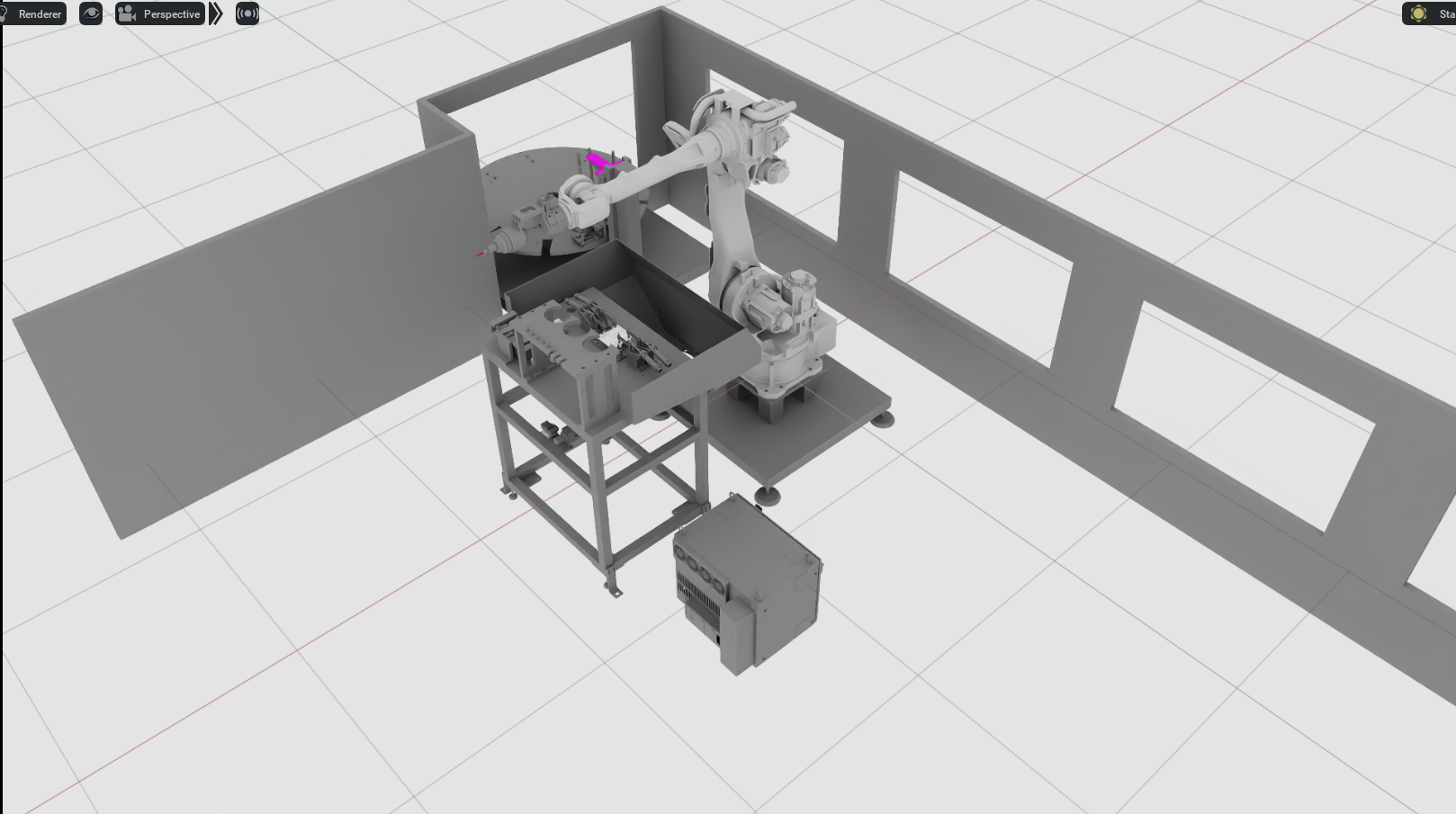
[Above] CAD files of the factory environment provided, [Below] Simulation environment generated from CAD

The problem is the gap between simulation and reality.

Ideal Assumptions in Simulation

• The robot is a perfect rigid body
• Joints have perfect axes of rotation
• No friction or backlash

Imperfections in Reality

Real robots have numerous error factors:

Kinematic Errors

• Minor differences between actual link lengths and CAD models due to manufacturing tolerances
• Joint axis misalignment due to assembly errors

Non-Kinematic Errors

• Robot arm deflection due to gravity
• Gear backlash
• Metal expansion/contraction due to temperature

These errors apply to all elements - the robot, end effector, and work environment - and accumulate.

Robot calibration is not simply coordinate setting. It is the technique of measuring imperfect physical parameters in reality and compensating the virtual model.

Comparison of Calibration Methods

Calibration methods used in industrial settings are divided into three categories based on precision requirements and cost.

1. Manual Teaching

The most intuitive method. An operator uses a teach pendant to directly contact the robot TCP (Tool Center Point) with objects to calculate the coordinate system.

Limitations:

• Result variation depending on operator skill (Human Error)
• Re-teaching required with every process change
• Difficult to ensure consistency

2. Vision Sensor-Based (Hand-Eye Calibration)

Uses cameras to recognize checkerboards or markers and converts coordinates through $AX = ZB$ matrix operations.

Advantages: Automatable, non-contact, fast measurement

Limitations:

• Additional errors from lens distortion
• Sensitive to lighting conditions
• Resolution degradation with distance

3. Precision Measurement Equipment (Laser Tracker, etc.)

Laser trackers can achieve precision below 1mm.

Limitations:

• Equipment costs of tens of thousands of dollars or more
• Installation environment constraints

Method	Advantages	Disadvantages	Precision
Manual Teaching	Intuitive, no additional equipment	Human Error, low reproducibility	1-3mm
Vision Sensor	Automatable, non-contact	Lighting/distortion variables	0.5-2mm
Laser Tracker	Very high precision	Expensive, installation constraints	<0.1mm

Initial Attempt: Limitations of ArUco Markers

Our first approach was the most versatile ArUco marker based method.

We detected marker corners with cameras and estimated 3D position and pose using the PnP (Perspective-n-Point) algorithm. This worked efficiently for existing Pick & Place tasks.

However, this project required sub-0.5mm ultra-precision.

Structural Limitations of Vision-Based Approaches

1. Detection Value Jittering

Measurement values constantly fluctuate due to subtle changes in lighting and sensor noise. Even statistical averaging cannot achieve sub-millimeter precision.

2. Inverse Relationship Between Distance and Resolution

To cover the robot's wide working radius, cameras must be placed far away. As distance increases, the actual distance per pixel increases, causing resolution to drop sharply.

We achieved precision around 1mm with the ArUco method, but sub-0.5mm was structurally impossible.

New Approach: Touch Probe + Kabsch Algorithm

Why We Chose Touch Probe

Introducing expensive laser trackers was impractical. We focused on the fact that "the most primitive method can be the most accurate".

Touch Probe Strengths:

1. Physical contact-based measurement - No lighting or lens distortion effects
2. Leverages robot repeatability - Industrial robot repeatability is at the 0.02-0.05mm level
3. Automated probing - Eliminates Human Error
4. Cost efficiency - Less than 1/10 the cost of laser trackers

Renishaw's Touch Trigger Probe provides 0.25um repeatability. Combined with robot repeatability, sub-millimeter calibration becomes achievable.

Kabsch Algorithm: Deriving Optimal Rotation Transform

We need to find the optimal transformation matrix between points measured with the Touch Probe and points in simulation.

The Kabsch Algorithm calculates the rotation matrix and translation vector that minimize RMSD (Root Mean Square Deviation) between two point clouds.

Optimization Problem Definition

Given two point clouds $P = \{\mathbf{p}_1, \mathbf{p}_2, ..., \mathbf{p}_N\}$ and $Q = \{\mathbf{q}_1, \mathbf{q}_2, ..., \mathbf{q}_N\}$:

$$\min_{R, \mathbf{t}} \frac{1}{2} \sum_{i=1}^{N} d(\mathbf{q}_i, R\mathbf{p}_i + \mathbf{t})^2$$

where $R$ is the rotation matrix and $\mathbf{t}$ is the translation vector.

Step 1: Centroid Calculation

Calculate the centroid of both point clouds:

$$\bar{\mathbf{p}} = \frac{1}{N} \sum_{i=1}^{N} \mathbf{p}_i, \quad \bar{\mathbf{q}} = \frac{1}{N} \sum_{i=1}^{N} \mathbf{q}_i$$

Generate centered point clouds:

$$\mathbf{p}'_i = \mathbf{p}_i - \bar{\mathbf{p}}, \quad \mathbf{q}'_i = \mathbf{q}_i - \bar{\mathbf{q}}$$

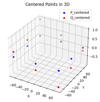
Centered point clouds of simulation positions (Q_centered) and actual environment positions (P_centered)

Step 2: Covariance Matrix Calculation

Calculate the $3 \times 3$ covariance matrix $H$ representing the correlation between the two point clouds:

$$H = P'^T Q'$$

where $P'$ and $Q'$ are $N \times 3$ matrices with centered points as rows.

Step 3: Singular Value Decomposition (SVD)

Decompose the covariance matrix $H$ using SVD:

$$H = U \Sigma V^T$$

• $U$: $3 \times 3$ orthogonal matrix
• $\Sigma$: Diagonal matrix containing singular values
• $V^T$: $3 \times 3$ orthogonal matrix

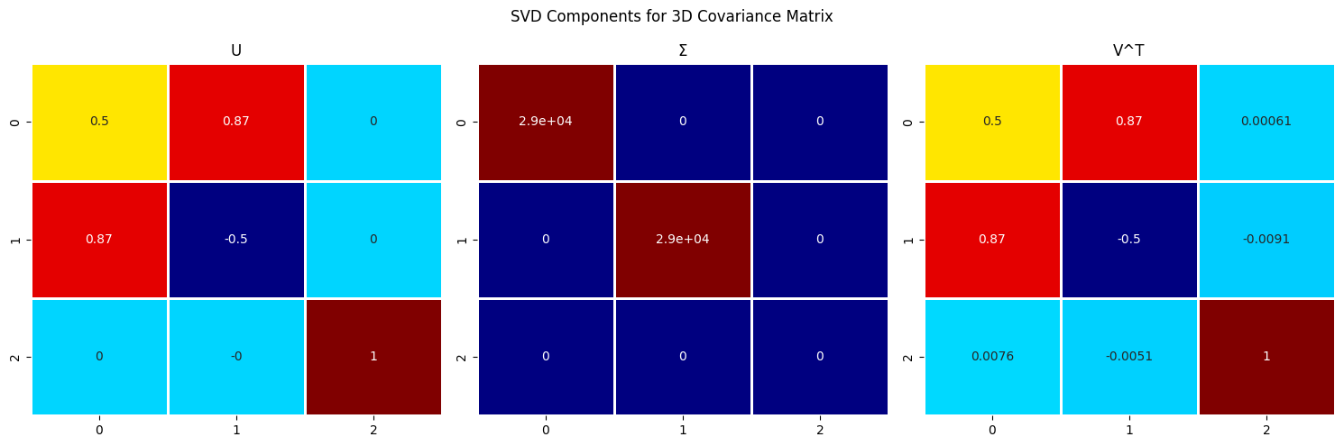
SVD decomposition results used in actual calculation

Step 4: Deriving the Optimal Rotation Matrix

Calculate the optimal rotation matrix $R$ from SVD results:

$$R = V U^T$$

Reflection Handling:

If $\det(VU^T) = -1$, reflection rather than rotation occurs. To correct this:

$$R = V \begin{bmatrix} 1 & 0 & 0 \\ 0 & 1 & 0 \\ 0 & 0 & d \end{bmatrix} U^T, \quad d = \text{sign}(\det(VU^T))$$

Step 5: Translation Vector Calculation

Calculate the optimal translation vector $\mathbf{t}$ from centroids:

$$\mathbf{t} = \bar{\mathbf{q}} - R\bar{\mathbf{p}}$$

Final Transformation Matrix

The $4 \times 4$ homogeneous transformation matrix combining rotation $R$ and translation $\mathbf{t}$:

$$T_{calib} = \begin{bmatrix} R & \mathbf{t} \\ \mathbf{0}^T & 1 \end{bmatrix}$$

Mathematical Optimality Guarantee

The Kabsch Algorithm mathematically guarantees the solution that minimizes RMSD:

$$\text{RMSD} = \sqrt{\frac{1}{N} \sum_{i=1}^{N} d(\mathbf{q}_i, R\mathbf{p}_i + \mathbf{t})^2}$$

where $d(\cdot, \cdot)$ is Euclidean distance.

Since the SVD-based solution provides a closed-form optimal solution, computation is fast compared to iterative optimization and there are no convergence issues.

Practical Application Results

Calculated Rotation Transform

Euler angles calculated by the Kabsch Algorithm in our project:

Axis	Radians	Degrees
Roll	0.005054	0.289582 deg
Pitch	0.007563	0.433337 deg
Yaw	-0.001171	-0.067092 deg

These are very small rotation errors, but at the robot arm's end effector, they amplify to several millimeters of position error.

Transform Application Results

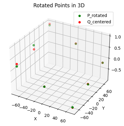
Aligned point cloud (P_rotated) after applying the rotation transform calculated by the algorithm

Overcoming the Sim-to-Real Gap

We fed the calibration matrix $T_{calib}$ back to the robot controller in real-time, precisely mapping paths generated in virtual simulation to the misaligned real environment.

Result: Achieved sub-0.5mm precision that was impossible with vision-based approaches

Implementation Code Example

import numpy as np
from scipy.spatial.transform import Rotation

def kabsch_algorithm(P: np.ndarray, Q: np.ndarray) -> tuple[np.ndarray, np.ndarray]:
    """
    Calculate optimal rotation matrix and translation vector using Kabsch Algorithm

    Args:
        P: Source point cloud (N x 3)
        Q: Target point cloud (N x 3)

    Returns:
        R: Optimal rotation matrix (3 x 3)
        t: Optimal translation vector (3,)
    """
    # Step 1: Centering
    centroid_P = np.mean(P, axis=0)
    centroid_Q = np.mean(Q, axis=0)

    P_centered = P - centroid_P
    Q_centered = Q - centroid_Q

    # Step 2: Covariance matrix
    H = P_centered.T @ Q_centered

    # Step 3: SVD
    U, S, Vt = np.linalg.svd(H)

    # Step 4: Rotation matrix (including reflection correction)
    d = np.sign(np.linalg.det(Vt.T @ U.T))
    R = Vt.T @ np.diag([1, 1, d]) @ U.T

    # Step 5: Translation vector
    t = centroid_Q - R @ centroid_P

    return R, t


def compute_rmsd(P: np.ndarray, Q: np.ndarray, R: np.ndarray, t: np.ndarray) -> float:
    """Calculate RMSD after applying transformation"""
    P_transformed = (R @ P.T).T + t
    return np.sqrt(np.mean(np.sum((Q - P_transformed) ** 2, axis=1)))


# Usage example
if __name__ == "__main__":
    # Simulation point cloud (Touch Probe measurement positions)
    P_sim = np.array([
        [100.0, 0.0, 50.0],
        [200.0, 0.0, 50.0],
        [150.0, 100.0, 50.0],
        # ... additional measurement points
    ])

    # Real environment point cloud (Touch Probe actual measurements)
    P_real = np.array([
        [100.12, 0.45, 49.87],
        [200.15, 0.52, 49.91],
        [150.08, 100.38, 49.82],
        # ... additional measurement points
    ])

    R, t = kabsch_algorithm(P_real, P_sim)
    rmsd = compute_rmsd(P_real, P_sim, R, t)

    # Extract Euler angles
    euler = Rotation.from_matrix(R).as_euler('xyz', degrees=True)

    print(f"RMSD: {rmsd:.4f} mm")
    print(f"Roll: {euler[0]:.4f} deg, Pitch: {euler[1]:.4f} deg, Yaw: {euler[2]:.4f} deg")
    print(f"Translation: {t}")

Key Takeaways

1. Sim-to-Real Gap is the greatest barrier to digital twin success. Kinematic and non-kinematic errors accumulate, creating gaps between reality and simulation.

2. Vision-based calibration is convenient but has structural limitations for processes requiring sub-millimeter precision.

3. Touch Probe is based on physical contact, unaffected by lighting/distortion, and enables automation leveraging robot repeatability.

4. Kabsch Algorithm mathematically guarantees the optimal transformation matrix that minimizes RMSD using SVD.

5. The combination of these two technologies enables sub-0.5mm Sim-to-Real calibration.

Precise calibration begins not with fancy equipment, but with choosing the right algorithms and measurement principles.